CHAPTER-19-F

NAVAL ORDNANCE AND GUNNERY
VOLUME 2, FIRE CONTROL

CHAPTER 19
SURFACE FIRE CONTROL PROBLEM

HOME INDEX
Chapter 19 SURFACE FIRE CONTROL PROBLEM
A. General
B. Analytical solution
C. Graphic rangekeeping
D. Mechanical solution-general
E. Basic mechanisms
F. Mechanical solution-basic rangekeepers
G. Mechanical solution-establishing the horizontal plane

F. Mechanical Solution-Basic Rangekeeper

19F1. General

The manner in which a computing instrument solves the surface fire control problem will be explained in this section, using the Rangekeeper Mark 8 as a model. This discussion is not to be considered a full presentation of the Rangekeeper Mark 8, which would be beyond the scope of this text; the student whose duties require more complete information is referred to the publications of the Bureau of Ordnance on the subject.

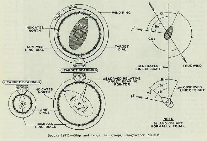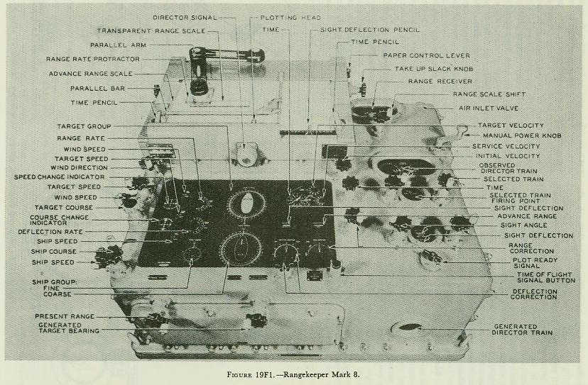
Figure 19F1 is a top view of the computing section of the Rangekeeper Mark 8, showing the arrangement of the various dial groups, knobs, and cranks. Figure l9F2 is a picture of the center dial groups, the upper dial indicating target course as well as wind direction; the lower dial showing own-ship course and target bearing. The line of sight from own ship to target is represented by the fixed indices, labeled “target bearing.” The dials thus give a visual picture of the own-ship and target set-up (which is vectorially represented to the right of the dials on the figure).

To clarify discussion, the rangekeeper may be considered to have three fundamental sections. This is a functional division of the rangekeeper rather than a physical one. The sections are:

1. The tracking section.

2. The prediction section.

3. The correction section.

19F2. Tracking section

The tracking section, given proper inputs, continuously provides the rates of change of range and bearing due to motion of own ship and target. It also generates present range, cR, and relative target bearing cBr. The target’s actual position relative to own ship is determined continuously by the director, which measures range and bearing. The generated values of range and bearing developed in the tracking section established a continuous value of present target position. When the rangekeeper is receiving the correct inputs, the actual target position and the generated position should be the same; this can be checked by comparing the actual and generated values of range and bearing.

19F3. Prediction section

Using values from the tracking section, the prediction section computes the position the target will occupy at the end of the time of flight. At the same time, this section computes the elevation and deflection offsets necessary to hit this predicted position in accordance with the range table and with existing variations from range-table standard conditions. The computation of these corrections is carried out in the ballistic part of the prediction section. The final step is to convert these predictions, including ballistics, into sight angle and sight deflection, the angular offsets from the line of sight which will position the gun to hit the target at the end of the time of flight.

19F4. Correction section

The correction section takes care of the effects of deck inclination. It has two parts, the trunnion-tilt corrector and the deck-tilt corrector. The trunnion-tilt corrector, as its name implies, corrects gun train and elevation for the tilting of the gun trunnions.

The deck-tilt corrector works out corrections to the line of sight to take care of deck inclination. The director measures the bearing of the target in the deck plane, but the computer works out its solution in the horizontal. Whenever the deck is tilted, these two values in the deck and horizontal planes will differ by the amount of the deck-tilt correction. The bearing in the horizontal plane is obtained by a differential which combines the bearing measured by the director with deck-tilt correction.

19F5. Rangekeeper computing mechanism

Having summarized in a few words the function of each major part of the rangekeeper, it will now be in order to return to each section of the instrument in turn for more detailed analysis. In the balance of this section of the chapter the intermediate quantities used in the development of gun orders will be considered as they are evolved from the original inputs to the computer. The ultimate purpose of the entire system is the computation of gun train order, B’gr, and gun elevation order E’g, the values which position the gun to hit the target.

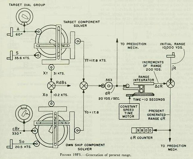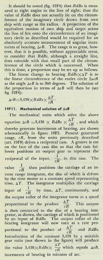
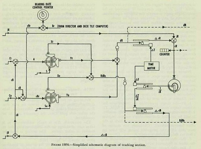
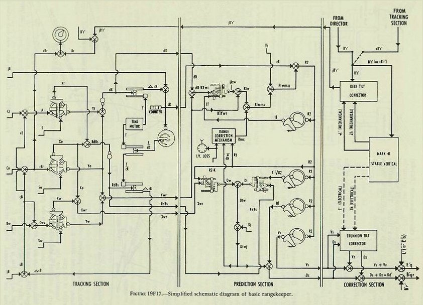
19F6. Range rate, dR

The range rate, dR, is the algebraic sum of the components of own-ship and target motion in the line of sight: expressed in symbols, dR=Yo+Yt. The arrangement by which this is accomplished in the rangekeeper is shown in figure 19F3. Values of target angle, A, and target speed, S, (initially estimated by the spotter) are cranked into the target-component solver. The outputs of this component solver are the target components in and across the line of sight (Yt and Xt respectively).

Own ship’s speed, So, which is received automatically from the pitometer log, is combined in the own-ship component solver with an input of relative target bearing. (The generated rather than observed value of target bearing is used, for reasons which will be explained later.) The resulting outputs are the own-ship components in and across the line of sight (Yo and Xo respectively). The components in the line of sight, Yo and Yt, are then added algebraically in a differential, as shown in the figure, to obtain range date, dR, expressed in knots. This quantity is next changed from knots to yards per second by means of a simple gear ratio. The value of dR also, through appropriate gearing, positions a counter on the face of the rangekeeper, and is used by the operator to compare with measured range rate and thus determine if correct set-up of the elements has been made.

19F7. Increments of generated range,

If some means is provided to multiply the rate of change of range by time as it elapses, the result will be a continuous set of increments of range in yards. A disc integrator, previously described, accomplishes this. The value of dR is used to posidon the carriage of the range integrator; the disc is revolved by a constant speed time motor. The resulting output of the integrator                   is increments of generated range,          which are constantly accumulated as shaft rotation.

19F8. Generated present range, cR

When the increments of generated range,          are added to the value of initial range, jR, as measured by the radar or rangefinder, the result will be generated present range, cR. Figure 19F3 shows how this is accomplished in the rangekeeper by means of a differential. The value of cR appears on a range counter on the face of the rangekeeper, except as noted in article 20E6 (4). It is also an important input to the prediction section.

19F9. Linear deflection rate, RdBs

Referring again to figure 19F3, it is seen that the deflection rate of the target, Xt, is an output of the target-component solver. The deflection rate of own ship, Xo, is provided by the own-ship component solver. These are added in a differential to produce the total linear deflection rate, RdBs. This is a linear rate in knots; it is then converted from knots to yards per second by means of a gear ratio.

19F10. Increments of bearing,

It would be possible to compute linear increments of bearing in yards by multiplying RdBs by increments of elapsed time in an integrator, as was done in the case of increments of range. Since, however, an angular rather than a linear bearing rate is needed for the purpose of evolving generated bearing, it is necessary that a means be provided in the rangekeeper to convert linear increments of bearing, found as described above, to angular increments expressed in angular units, such as minutes of arc.

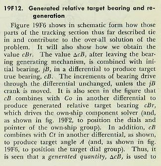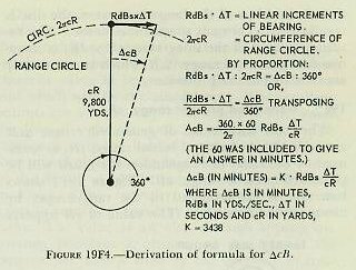
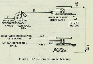
position the course gears of the own-ship and target-component solvers. This means that once the problem has been solved, this quantity,
drives back continuously to reposition the component solvers in accordance with the development of the relative-motion problem. This process is called regeneration, and is one of the most important features of the rangekeeper. Because of this regenerative feature, the rangekeeper is able to handle the indirect fire problem and, in fact, is able to continue to compute gun orders during any period when the director cannot see the target. Should the target change course or speed during such periods, of course inaccurate gun orders will result.

19F13. Summary of tracking section

The values supplied to the tracking section were (1) the known elements, So and Co; (2) the measured elements, jR and jB; and (3) the estimated elements, A and S. From these it has developed generated rates, dR and RdBs, and increments, which have been used to determine the generated quantities cR and cB. Comparison of these generated values with the observed values transmitted from the director provides the rangekeeper operators with a method of checking the solution; i. e., of checking the estimates used for the values of A and S. This feature of operation, known as rate control, will be further developed in article 20E7 of the next chapter.

The outputs of the tracking section, dR, cR, and RdBs, become inputs to the prediction section, which makes use of them in the computation of sight angle and sight deflection.

19F14. Prediction of sight angle, Vs

Sight angle, as computed by the rangekeeper, includes the corrections for four quantities; namely, relative motion during time of flight, range wind, initial velocity loss, and a quantity known as range error due to deflection. Sight angle is computed in the vertical plane, and the assumption is made
that the gun and target are in the same horizontal plane; that is, target elevation is assumed to be zero. Sight angle is merely the angular equivalent, in minutes of arc, of advance range in yards.

Advance range differs from the actual range to the advance position of the target by the ballistic corrections. To compensate for factors such as own-ship motion, target motion, wind, and variations in initial velocity, the gun must be elevated for a range equal to present range plus the algebraic sum of the several range compensations. During the time of flight, the target will travel to the computed point of fall shown, and the projectiles will hit. The equation for advance range is R2=cR+Rj+Rtwmx.

Present range cR, was generated in the tracking section. Rj, range spot, is entered into the rangekeeper as sent down from the director. It is now necessary to consider the several elements comprising Rtwmx and show how each is computed in the prediction section of the rangekeeper. The prediction Rtwmx is the sum of the following elements:

1. Rt-the range prediction to compensate for relative target motion during the time of flight, Tf. Relative target motion includes own-ship motion. It will be recalled that own-ship’s motion imparts additional velocity to the projectile, which is the effect here considered. Obviously any motion of own ship after the projectile leaves will have no effect on the projectile’s travel.

2. Rw-the range prediction to compensate for the effect of apparent wind on the projectile.

3. Rm-the range prediction to compensate for variations from the designed initial velocity.

4. Rx-the range prediction to compensate for the effect of deflection exclusive of drift.

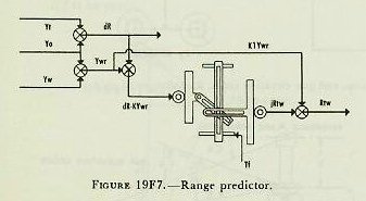19F15. Range prediction, Rtw

The predictions to compensate for relative target motion and for wind are made in a multiplier called a range predictor (see fig. 19F7). If dR, the range rate, is multiplied by Tf, the result will be the relative motion in range during the time of flight. Since own-ship and target motion are added together to form dR, wind due to own ship’s motion must be handled separately. This is done by using apparent wind, a fictitious value which combines vectorially the true range wind and the range wind due to own ship’s motion. True-wind direction and velocity are set in the rangekeeper, the outputs of the wind-component solver being Yw and Xw, components of true-wind velocity in and across the LOS. Since apparent wind is the resultant of own-ship motion reversed and true-wind motion, range components of these elements are then combined in a differential, the output of which is Ywr, the component of apparent wind velocity along the line of sight (Ywr=Yo+ Yw).

Instead of multiplying dR and Ywr by Tf separately, it is simpler to combine them and eliminate one multiplier. In computing Rtw (Rt+Rw), an empirical equation Rtw=Tf (dR-KYwr)+K1Ywr must be used, since Tf X Ywr alone will not produce the change in range caused by range wind (Ywr).

Referring again to figure 19F7, it is seen that range rate dR and apparent range wind Ywr are combined in a differential to give dR-KYwr, and this output is then multiplied by Tf to give jRtw, to which K1Ywr is added in a differential to give Rtw, the range prediction due to relative target motion and apparent range wind during the time of flight.

19F16. Range correction for I. V. loss and deflection exclusive of drift, Rmx

Referring to the schematic diagram of the prediction section, figure 19F10, it can be seen that Rtw, computed above, goes into a differential. Into the other side goes Rmx, the quantity now to be considered.

The correction Rm is easily understood, as it takes care of change in the initial velocity due to erosion or other causes. The setting is made by the initial-velocity knob and dial, which introduces jRm as shown in figure l9F9.

The need for correction Rx is not so apparent and can best be shown by a simplified example. In figure l9F8, own ship is shown to be motionless and the target is moving to the right from position 1 at the instant of firing to position 2 at the end of the time flight. At position 1 target angle is assumed to be 90 degrees; range rate therefore is zero. It is also assumed for simplicity that there is no wind blowing and that the projectile leaves the guns at the design value of initial velocity.

Since dR is zero when the target is at position 1, the range prediction (Rt) will also equal zero and the value of advance range will be equal to present range. With the guns elevated for present range and deflected to compensate for the target’s rightward motion during the time of flight, it is obvious from the diagram that the salvo will fall short by the amount Rx.

This error is the result of computing the range prediction from an instantaneous value of dR which is based on the present line of sight; whereas dR will actually be a changing value if Br and A Care changing during the time of flight. It will be noted that drift is excluded in the computation of Rx. The reason for this is that when the data for the various range tables are collected at the proving grounds, the range error caused by drift is compensated for. For instance, when a test round is fired at a gun elevation of 20 degrees, the range to the point of fall is actually measured, and any loss of range due to drift is thus taken care of in the range-table values.

From figure 19F9, it can be seen that drift, Df, is subtracted from total sight deflection, Ds, leaving Dtwj; that is, deflection exclusive of drift, and empirically jRx equals K (Dtwj)2. jRx is added to jRm to give jRmx, which is one input to the range-correction multiplier, the other input being R2. The output is Rmx.

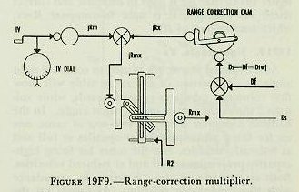
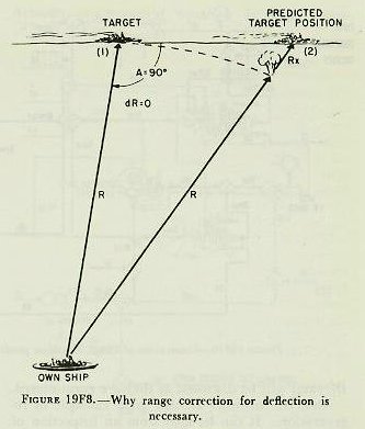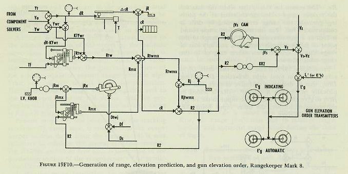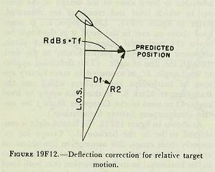
19F17. Total range correction, Rjtwmx

As shown in the schematic, figure 19F10, range prediction Rtw, is now combined with range correction, Rmx, in a differential to give Rtwmx. Range spot, Rj, if any, is then combined with Rtwmx in another differential, the output of which is total range correction, Rjtwmx.

19F18. Advance range, R2

From the schematic, figure 19F10, it can be seen that advance range, R2, is obtained by adding the total range correction, Rjtwmx, to the present generated range, cR, driven in from the tracking section. It should be recalled that advance range, R2, is not equal to the actual range to the target’s predicted position, the difference being due to the ballistic corrections for I. V. loss, range correction due to deflection, wind, and range spots. These corrections are included to ensure that the gun will be elevated the proper amount to hit the predicted position. If not included, the effects mentioned above would cause the projectile to fall short of or over the predicted position. Although R2 is a fictitious value and not the actual range to the target’s predicted position, when this range is converted into sight angle and applied at the guns, the result should be a gun elevation which will cause hits on the target.

As shown in the schematic, R2 is used for several purposes in the prediction section. The most important use is its conversion by means of a cam into its equivalent angular value, sight angle Vs, which is used in making up gun elevation order and for setting the sights at the guns. R2 is also a necessary input to the range-correction mechanism. Other uses of R2 in the deflection part of the prediction section (namely as inputs to the wind-deflection multiplier, the Tf /R2 cam, and the drift, Df, cam) will be discussed as they are encountered. Also, R2 furnishes another good example of regeneration. It can be seen from an inspection of figure l9F10 that R2 is used to compute and correct itself; for example, it is used to compute Rmx, which became part of R2.

19F19. Sight angle, Vs

As mentioned above, R2 is used to compute sight angle Vs. Inspection of any range table will show that column 1 tabulates range in yards, while column 2 shows the corresponding sight angle. In the ballistic computer there are two sets of cams, one set for firing armor-piercing projectiles at full and at reduced velocities, and the other for firing high-capacity projectiles at full and at reduced velocities. Both sets are designed to function in accordance with this range-table relation. As shown on the schematic, R2 rotates the Vs cam and computes jVs, a partial correction, while R2 in a gear train computes KR2, the straight-line function. When combined in a differential, jVs+KR2=Vs. This value is now ready to be used in making up gun-elevation order.

19F20. Prediction of sight deflection

The next step to be considered is the computation of sight deflection, Ds, the angular amount which the bore of the gun must be offset in the horizontal plane from the LOS. This quantity is made up of the following elements.

1. Dt-deflection prediction to compensate for relative target motion in deflection during the time of flight.

2. Dw-deflection prediction to compensate for the effect of apparent wind on the projectile during the time of flight.

3. Df-deflection prediction to compensate for drift.

4. Dj-manual deflection correction (spots).

19F21. Deflection prediction for relative motion, Df

We have already studied the computation of RdBs, linear deflection rate due to relative motion of own ship and target, also the computation of advance range R2, and of Tf corresponding to advance range. If RdBs and Tf are multiplied, the result will be the linear deflection (in knots, which can be converted to yards per second by a gear ratio) due to own-ship and target motion. As has been stated, it is easier to visualize this motion if own ship is considered stationary and the combined motion of own ship and target are represented as target motion, as is done in figure l9Fl2.

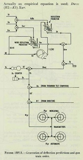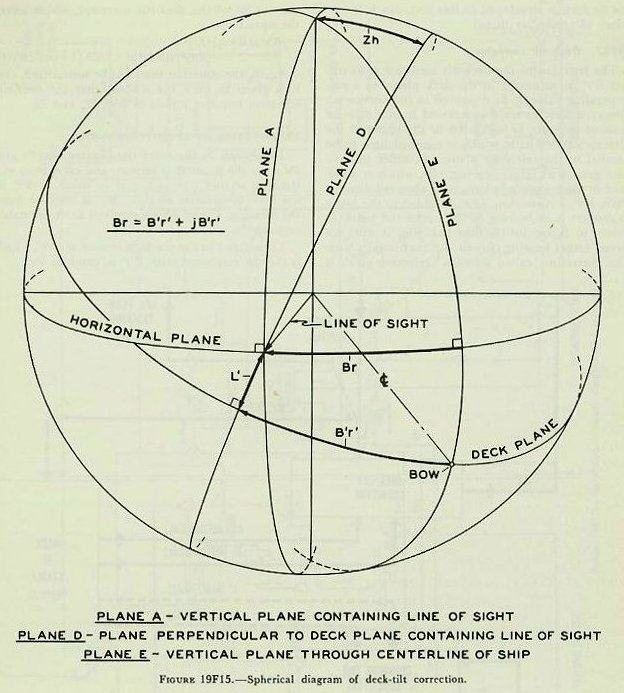
When RdBs X Tf is known, the predicted position of the target at end of Tf is determined. However, to direct the guns, angular deflection from the LOS, Dt, is needed. In order to convert from linear to angular measure, advance range R2 must be considered, because the angular prediction varies with range and becomes larger as range decreases. The formula employed is similar to that described in connection with generation of increments of bearing. The equation is:

Dt=3,438 x RdBs x Tf/R2; in which

Dt is in minutes,
RdBs is in yards per second,
Tf is in seconds, and
R2 is in yards.

Reference to the schematic, figure l9Fl3, shows how the rangekeeper solves the above equation mechanically. The linear deflection rate RdBs, from the tracking action, is multiplied by Tf/R2 in the deflection-prediction multiplier to produce Dt. The constant K (3,438) is introduced by a gear ratio (not shown). After establishment of Dt, the angular prediction for relative motion, corrections must be made for wind and drift.

19F22. Correction for wind, Dw

Deflection prediction to compensate for the effect of apparent wind on the projectile, Dw, is computed in a multiplier known as the wind-deflection predictor. Xo (reversed) and Xw are added algebraically in a differential to give Xwr, the component of apparent wind velocity across the line of sight. This is multiplied by R2 to give Dw.
Actually an empirical equation is used; Dw= (R2-Kl) Xwr.

The quantities Dw and Dt enter a differential to produce Dtw, as shown in figure 19F13. Deflection spot, Dj, if any, is applied by handcrank to make Dtwj. It will be recalled that Dtwj is used in the range correction mechanism to compute Rx, the range correction for deflection exclusive of drift.

19F23. Correction for drift, Df

The angular correction for drift increases as range increases; and, since this correction Df is very nearly proportional to advance range R2, Df is shown in the schematic, figure 19F13, as being produced by a gear ratio from an input of sight angle Vs. Df=(K-K1)Vs.

NOTE: Actually drift, Df, and TJ vary with R2 and are nearly proportional to Vs. In the rangekeeper the sight-angle cam output, Vs, after passing through suitable gearing, is used for Df and Tf/R2.

Df is added to Dtwj in a differential to produce sight deflection Ds; this value is now ready to be used in the computation of gun train order.

19F24. Summary of prediction section

The inputs to the prediction section were dR, cR, RdBs, Xwr, and Ywr from the tracking section as described previously, and a manual input of I. V. loss. In addition the prediction section receives any range and deflection spots which may have been made. The resultant outputs are Ds and Vs; these quantities are sent to the gun mounts for the purpose of setting the gun sights.

If it were not for the roll and pitch of the ship, gun orders could be made up simply by adding the computed values of sight angle and sight deflection to director elevation and director train, as shown in figures 19F1 and 19F14, thus:

E’g=E’b + Vs.

B’gr=B’r’+Ds.

It will be noted that these equations not only assume a level deck, but also disregard corrections for parallax and roller-path inclination. This is justified by the fact that, in surface systems, the necessary corrections for these errors are made in instruments located at the directors and gun mounts, rather than in the rangekeeper.

Since the deck plane is rarely level, Vs and Ds, in addition to being used in computation of gun orders, must also be sent as inputs to the correction section, where with other values they form the basis of the correction necessitated by the inclination of the deck.

19F25. Level and crosslevel

Before considering in any detail how the two correctors in the correction section function, it is advisable to learn some of the details of the manner in which level and crosslevel are measured. Refer to figure l9Fl5. Level angle, L’, is measured about an axis in the deck; it is the angle between the horizontal plane and the deck plane, measured in the plane perpendicular to the deck through the line of sight. (This definition applies to level angle, L’, as measured in main-battery systems of battleships and cruisers which use the Rangekeeper Mark 8. It does not apply to level angle, L’ as used in the Computer Mark 1 for certain dual-purpose battery installations.)

As shown in figure 19F15, the line of sight is considered to be in the horizontal. Except for extremely short range, this assumption introduces no error. The deck plane is shown tilted with respect to the horizontal in such a direction that both level and crosslevel angles exist. By the definition of level angle (L’) above, L’ is measured in plane D-the plane perpendicular to the deck plane containing the line of sight-and it is the angle between the deck plane and the horizontal measured about an axis in the deck normal to plane D.

Crosslevel, Zh, is measured about the axis in the horizontal plane where the horizontal plane and the vertical plane containing the line of sight intersect; it is the angle between the vertical plane (plane A) and a plane perpendicular to the deck (plane D) through the axis just defined above.

19F26. The trunnion-tilt corrector

The trunnion-tilt corrector is installed in the Rangekeeper Mark 8 for the purpose of computing corrections to gun elevation order and to gun train order caused by the depression of one trunnion below the other. Referring to article 19B12, it will be recalled that, when the trunnion axis leaves the horizontal, the gun will elevate in a plane other than the vertical, and that the effective elevation above the horizontal will be less than Vs. A deflection error is also introduced, the effects of which are generally more serious than the elevation error. The trunnion-tilt corrector provides the necessary elevation correction Vz, and the train correction Dz, which are used in the rangekeeper as shown in figure 19F16.

The Stable Vertical Mark 41, which supplies the values L’ and Zh, will be taken up in the next section. The trunnion-tilt corrector computes Dz and Vz by solving the equations:

These equations are given merely to show the values entering into solution of Vz and Dz. They will not be further developed in this text, nor is it necessary to remember them.

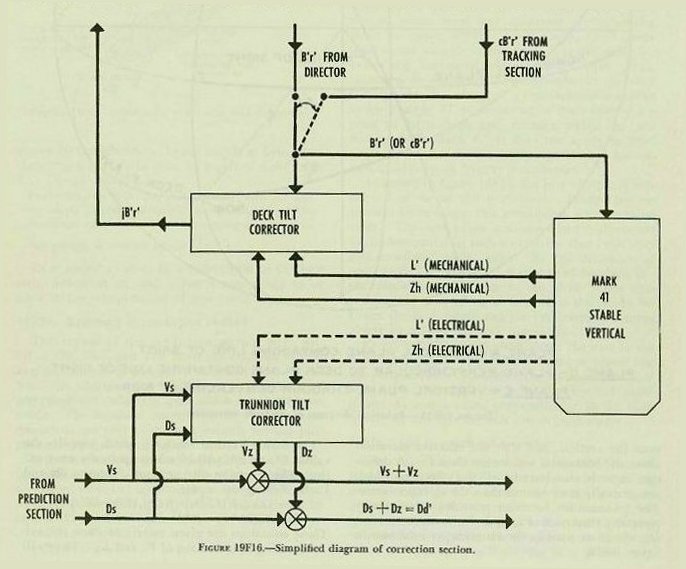19F27. Deck-tilt corrector

The function of the deck-tilt corrector is to correct B’r‘, as measured in the deck plane, to a corresponding value of Br measured in the horizontal. Observed director train as received from a director must of necessity be measured in the plane of the director’s roller path, which is assumed here to be parallel to the reference plane. In order to compare generated target bearing, cBr, which is measured in the horizontal plane, with observed director train, B’r‘, a correction, jB’r', is added to the latter to convert it to bearing in the horizontal plane as shown in figure l9Fl6, thus changing it into observed target bearing, Br, in the horizontal plane. The correction, called deck-tilt correction jB’r’, is the output of the deck-tilt corrector, which solves the equation:

Again, the equation need not be memorized, and it is given to show the student that the deck-tilt corrector requires inputs of B’r‘, L’, and Zh.

19F28. Summary of correction section

The inputs to the correction section are Vs and Ds from the prediction section, and cB’r' from the tracking section (the last used in place of B’r‘ in the full regenerative set-up). B’r‘ is received from the director; L’ and Zh are received from the stable vertical.

The output to the tracking section is jB’r’, which is therein combined with B’r‘ to produce Br.

The other outputs of this section are (Vs+Vz) and Dd’ which equals (Ds+ Dz). These quantities can now be used to compute gun orders which will be accurate with the deck tilted. The equations given in paragraph 19F24, when modified to obtain corrections for tilt, are as follows.

E’g=E’b+ Vs+Vz.
B’gr= B’r’+Dd’.

These expressions assume that the elements of the system are aligned to the reference plane, and that there is no parallax. Corrections for roller-path tilt and parallax are discussed in the next two articles, which summarize all quantities making up gun orders.

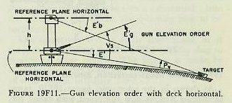
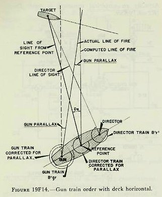
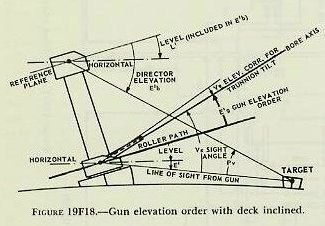
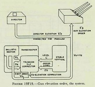
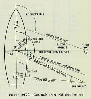
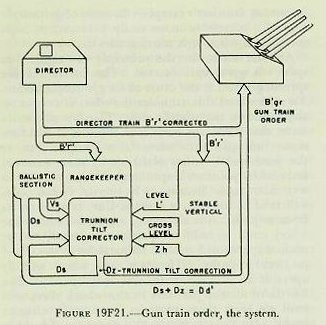
19F29. Gun elevation order

Gun elevation order is based on the elevation of the director pointer’s line of sight to the target, and is made up as shown in figure 19F18. This situation represents the most general case; that is, one which includes the most variables.

The director, when the sight is kept on the target, measures director elevation, E’b, which, with the deck inclined, includes level L’. E’b is corrected for vertical parallax and for director roller-path tilt to form the first element of gun elevation order, target position relative to the reference plane, measured from a reference point at the height of the gun.

Assuming for the moment that the gun roller path is parallel to the reference plane, all angles at the gun may be measured from the gun roller path, which represents zero gun elevation. Referring to figure 19F18, it can be seen that the angle level (L’) in effect reestablishes the horizontal plane. Measured below this is the angle E’, target elevation from the horizontal, which establishes a line of sight to the target from the reference point at the gun. Of course, the angles L’ and E’ do not exist separately in the mechanism; they are transmitted together in the form of director elevation E’b (i. e., E’+L’) corrected for vertical parallax. This value, E’b, is the first basic element, present position of the target relative to the deck.

At this point the gun has received a signal which, when laid off from its roller path, gives a line of sight to the target. Now, if sight angle Vs is added to this signal, it can be seen in the figure that a gun position above the line of sight to account for predictions and ballistics is established. As has been previously mentioned, although Vs is computed to produce a hit on a target in the same horizontal plane as the gun, a slight depression E’ below that plane will not create a measurable error, in accordance with the principle of rigidity of trajectory.

The gun-bore position above the line of sight must be corrected for trunnion tilt by the value Vz. The total angle of the bore axis above the roller path is gun elevation order, E’g. Since the roller path may not actually lie in the reference plane, the roller-path tilt corrector at the gun makes the necessary correction for this discrepancy. Figure 19F18 shows E’g as a composite angle, measured from the gun roller path, and made up of each of the corrections discussed above.

Figure 19F19 is a diagram of the director, range-keeper, stable vertical, and guns, in which the origin of the various quantities is shown. These quantities are actually combined within the range-keeper, but they have been shown outside for clarity.

19F30. Gun train order

Gun train order is shown diagrammatically in figure 19F20. Director train, B’r’ establishes the target position relative to ship’s centerline, measured in the deck plane. A non-reference director will include a horizontal parallax connector, which will cause the director to transmit director train for parallax, which in effect establishes a line of sight from the reference point, as in figure 19F20. This gives present position of the target relative to ship’s centerline and in the deck plane.

Measured from the fictitious line of sight from the reference point, sight deflection, Ds, is applied to account for predictions and ballistics, as can be seen in figure 19F20. Ds is computed in the horizontal plane, but if crosslevel is present the trunnion-tilt train correction, Dz, is added to produce the computed line of fire from the reference point. The sum of these angles is the angle that the computed line of fire makes with own ship’s centerline; that is, gun-train order, B’gr, in the deck plane. Gun train order is transmitted to the guns, where the proper horizontal parallax correction is applied to produce actual gun train to hit the target.

Figure 19F21 is a diagram of the gun train system. Although gun train order is actually made up within the rangekeeper, certain basic quantities are shown combined outside for clarity. As shown in figure 19F21, director train, B’r’ corrected for horizontal parallax, is received by the rangekeeper. It also is transmitted to the stable vertical to keep the gimbals oriented with the line of sight, so that the stable vertical can measure the values of level and crosslevel in the proper planes. Director train, B’r’, establishes present position of the target, measured from own ship’s centerline in the deck plane.

The prediction section computes sight deflection, Ds, in the horizontal plane, to account for relative motion and deflection ballistics.

The train correction, Dz, for trunnion tilt is computed in the trunnion-tilt corrector. This value accounts for the effect of crosslevel on the gun bore. Dz is added to Ds to produce deck deflection, Dd’, and this in turn is added to B’r‘ to produce gun train order, B’gr, in the deck plane, which is then corrected for horizontal parallax at each gun.